Special thanks to Yan Shuo Tan, who wrote most of this section’s content.
Review and introduction
To briefly recap what we have learnt so far:
We defined a superpopulation model, i.e. a distribution for :
is the (binary) treatment decision,
and are the potential outcomes in the universes where the unit wasn’t/was treated,
is a confounding variable (in other words, it has a causal effect on and on ) So far, we haven’t needed to make any assumptions about the distribution of these variables in general (only that it exists).
We defined our quantity of interest, the average treatment effect (ATE): , which tells us the average effect of the treatment. We saw that this is impossible to estimate unless we make further assumptions.
We saw that in a randomized experiment, we have the following:
The treatment decisions are random, and therefore are independent of the potential outcomes.
In other words, .
In this section, we’ll investigate how we can estimate the ATE in situations where we have unknown confounding variables. We’ll rely on natural experiments to help us. Note that you’ve probably seen natural experiments before in Data 8, when learning about John Snow’s study of cholera.
Linear structural model (LSM)
In some fields (such as economics), it is typical to work with structural models, which place some restrictions on the joint distribution of all the variables, and in doing so, make it easier to estimate the parameters of the model.
We will work with the linear structural model relating our outcome to our treatment and confounding variable(s) :
where has mean zero, and is independent of and (in economics, we say that is exogenous). We sometimes further assume that , but this is not necessary for any of the analysis we’re going to do.
Note: in general, we often add the further structural equation where is an exogenous noise variable, and encodes the structural relationship between and . We won’t go into this level of detail, but when reading this equation, you should assume that is not necessarily 0.
This is not quite the same as the linear model that we have seen when we learned about GLMs, and that you’ve seen in previous classes! While it looks very similar, the linear model we worked with before is a statement about associations and predictions, while this linear structural model is a statement about intervention and action.
Specifically, this model assumes that if for unit , if we could set , we will observe , and if we could set , we will observe . (If is not binary, then there will be a potential outcome for each possible value of .) This is a subtle but important point, that also situates the linear structural model as a special case of the potential outcomes framework!
From this, we see that the average treatment effect in this model is (can you show this is true?), and furthermore, that the individual treatment effect for every unit is
In other words, the linear structural model is making an implicit assumption that the treatment effect is constant across all units.
Causal graphs and LSMs
Apart from the causal effect of on , the linear structural model also does something new from before. It asserts the causal relationships between the other variables, i.e. it tells us how and change if we manipulate .
The above linear structural model can be represented graphically as follows:
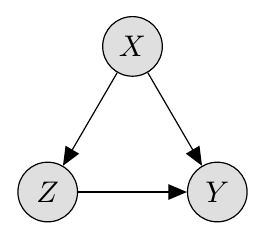
As a reminder, the arrows from into and assert that causes both and (i.e. intervening on changes the values of and ), and the arrow from into asserts that causes .
Confounding and omitted variable bias
In many scenarios, confounding is complicated and involves many different variables, and it may be impossible to collect, observe, or describe all of them. In that case we must assume that is unobserved. If this happens, then just as before, we’re in trouble because of confounding. Here are some examples. In each one, we’ve only listed one possible confounder , but there are likely many more: can you think of at least one for each example?
| Treatment | Outcome | Possible confounder(s) |
|---|---|---|
| Health insurance | Health outcomes | Socioeconomic background |
| Military service | Salary | Socioeconomic background |
| Family size | Whether the mother is in the labor force | Socioeconomic background |
| Years of schooling | Salary | Socioeconomic background |
| Smoking | Lung cancer | Socioeconomic background |
Note that in most of these examples, socioeconomic background is a confounder. This is particularly common in economics and econometrics, where most of the methods in this section originated.
Let’s be a bit more precise about quantifying the effect of confounding. Specifically, we’ll assume the linear structural model above, and then see what happens when we naively try to fit a linear regression to using , without accounting for .
Let be the solution of the least squares problem . We then get
The second term is a bias in the estimator: in other words, it’s the difference between the true value and the estimator, and it depends on the omitted (i.e., unobserved) variable . So, we’ll call this term the omitted variable bias.
Remark: is the infinite population version of the typical formula , where we now use and to denote matrices/vectors.
Why can’t we just adjust for confounding? Having such confounders is problematic because in order to avoid omitted variable bias, we need to have observed them, and added them to our regression (collection of such data may not always be feasible for a number of reasons.) Furthermore, there could always be other confounders that we are unaware of, which leaves our causal conclusions under an inescapable cloud of doubt.
Instrumental Variables
Is there a middle way between a randomized experiment and assuming unconfoundedness, which is sometimes unrealistic?
One way forward is when nature provides us with a “partial” natural experiment, i.e. we have a truly randomized “instrument” that injects an element of partial randomization into the treatment variable of interest. This is the idea of instrumental variables. We will first define the concept mathematically, and then illustrate what it means for a few examples.
Definition: Assume the linear structural model defined above. We further assume a variable such that , with (relevance), independent of , and (exogeneity). Such a is called an instrumental variable.
Remark: This replaces the earlier equation from before that .
Let us now see how to use to identify the ATE .
Where the second equality follows from the exogeneity of . Meanwhile, a similar computation with and gives us
Putting everything together gives
In other words, is the ratio between the (infinite population) regression coefficient of on , and that of on .
This motivates the instrumental variable estimator of the ATE in finite samples:
where again, abusing notation, , and refer to the vectors of observations. If , then this is a plug-in estimator of , and is consistent.
Further interpretation for binary : When is binary, we can show that
Hence, we can think of IV as measuring the ratio of the prima facie treatment effect of on and that of on .
Causal graph for instrumental variables
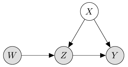
The relationships between , and can be represented as the following causal graph:
 />
/>
How to read this graph:
The arrow from into shows that has a causal effect on
The absence of any arrow into means that is exogeneous, i.e. no variable in the diagram causes , and in particular is independent of .
The absence of an arrow from into means that the only effect of on is through .
We shaded in , and because these nodes are observed, but is unshaded because it is latent (unobserved).
Note that we do not need to know or even be aware of what is in order for instrumental variables to work! It doesn’t matter how many confounders there are, or whether we’re even able to list all of them: as long as we can guarantee that they do not have any causal relationship to the instrument (exclusion restriction), instrumental variables will work.
Examples of instrumental variables
Let’s examine what we might use as instrumental variables for the five examples from the table in the previous section. The first four are taken from the econometrics literature:
Example 1: is health insurance, is health outcomes, is socioeconomic background. Baicker et al. (2013) used the 2008 expansion of Medicaid in Oregon via lottery. The instrument here was the lottery assignment. We previously talked about why this was an imperfect experiment because of compliance reasons (only a fraction of individuals who won the lottery enrolled into Medicaid), so IV provides a way of overcoming this limitation.
Example 2: is military service, is salary, is socioeconomic background. Angrist (1990) used the Vietnam era draft lottery as the instrument , and found that among white veterans, there was a 15% drop in earnings compared to non-veterans.
Example 3: is family size, is mother’s employment, is socioeconomic background. Angrist and Evans (1998) used sibling sex decomposition (in other words, the assigned sexes at birth of a sibling) as the IV. This is plausible because of the pseudo randomization of the sibling sex composition. This is based on the fact that parents in the US with two children of the same sex are more likely to have a third child than those parents with two children of different sex.
Example 4: is years of schooling, is salary, is socioeconomic background. Card (1993) used geographical variation in college proximity as the instrumental variable.
Example 5: is smoking, is lung cancer, is socioeconomic background. Unfortunately, this example does not lend itself well to an instrumental variable: despite decades of searching, nobody has yet found one that is convincing. This leads to an important lesson: not every problem is amenable to the use of instrumental variables, or even natural experiments!
As we see in these examples, sometimes you need to be quite ingenious to come up with an appropriate instrumental variable. Joshua Angrist, David Card, and Guido Imbens, who is named in several of these examples, are phenomenally good at this: in fact, they won the Nobel Prize in economics for their collected body of work!
Extensions
Multiple treatments / instruments, and two-stage least squares.
So far, we have considered scalar treatment and instrumental variables and . It is also possible to consider vector-valued instruments and treatments. To generalize IV to this setting, we need to recast the IV estimator in the previous sections as follows.
First define the conditional expectation , and observe that .
If we regress on , the regression coefficient we obtain is $$
$$
Here, the 2nd equality holds because is independent of all and , while the 4th equality holds because of a property of conditional expectations (one can also check this by hand by expanding out .)
In finite samples, we thus arrive at the following algorithm:
Two-stage least squares algorithm (2SLS):
Step 1: Regress on to get .
Step 2: Regress on to get .
For the scalar setting, it is easy to see that , but the benefit of this formulation is that it directly applies for vector-valued and .
(Optional) A non-parametric perspective on instrumental variables
In this notebook, we have introduced instrumental variables in the context of structural linear models. What if our model is nonlinear?
In an amazing coincidence, for binary treatment , the expression
has a meaning beyond the linear model setting. This is the subject of this groundbreaking paper by Angrist and Imbens in 1996.