Graphical Models, Probability Distributions, and Independence¶

Graphical Models¶

A graphical model provides a visual representation of a Bayesian hierarchical model using. These models are sometimes known as Bayesian networks, or Bayes nets.

We represent each random variable with a node (circle), and a directed edge (arrow) between two random variables indicates that the the distribution for the child variable is conditioned on the parent variable. When drawing graphical models, we usually start with the variables that don’t depend on any others. These are usually, but not always, unobserved parameters of interest like $\theta$ in this example. Then, we proceed by drawing a node for each variable that depends on those, and so on. Variables that are observed are shaded in.

We’ll draw graphical models for the three examples we’ve seen in previous sections: the product review model, the kidney cancer model, and the exoplanet model.

Graphical model for product reviews¶

In our product review model, we have the following random variables:

In this case, this means we start with a node for the product quality $\theta$, and then with one node for each review $x_i$, all of which depend on $\theta$. The nodes for the observed reviews $x_i$ are shaded in, while the node for the hidden (unobserved) product quality $\theta$ is not:

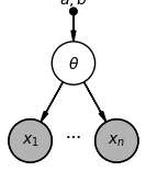
This visual representation shows us the structure of the model, by making it clear that each review $x_i$ depends on the quality $\theta$. But just as before, this model is simple enough that we already knew that. Next, we’ll look at the graphical model for a more interesting example.

Graphical model for kidney cancer death risk¶

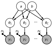
Recall the full hierarchical model for the kidney cancer death risk example:

• $y_i$ represents the number of kidney cancer deaths in county $i$ (out of a population of $n_i$).

• $\theta_i$ represents the kidney cancer death rate for county $i$.

• $a$ and $b$ represent the parameters of the shared prior for the county-level rates.

In order to draw the graphical model, we need to draw one node per random variable, and draw arrows to indicate dependency. We know that:

• We need a node for $a$ and a node for $b$.

• We need one node for each $\theta_i$ and one node for each $y_i$.

• Each $\theta_i$ depends on $a$ and $b$.

• Each $y_i$ depends on $\theta_i$ and $n_i$.

• Because $n_i$ is a fixed number, we’ll draw it as a dot.

So, our full graphical model looks like:

(Optional) Example: Graphical Model for Exoplanet Model¶

Text coming soon: see video

Relating graphical models to probability distributions¶

When we were drawing graphical models above, we drew one node per variable, and started from the “top,” working with the variables that didn’t depend on any others. We then worked our way through the model, ending with observed variables. When looking at a graphical model to derive the corresponding joint distribution of all the variables in the model, we follow a similar process. For example, in the kidney cancer death rate model, we can write the joint distribution of all the variables in our model by starting at the root (i.e., the nodes that have no parents), and then proceeding through their children, writing the joint distribution as a product.

So, we start with $p(a)$ and $p(b)$, then $p(\theta_i | a, b)$ (for $i \in \{1, \ldots, C\}$), then $p(y_i | \theta_i)$:

Factoring the distribution this way helps us understand and mathematically demonstrate the independence and dependence relationships in our graphical models, as we’ll see shortly.

Independence and Conditional Independence¶

Review: independence and conditional independence¶

We say that two random variables $w$ and $v$ are independent if knowing the value of one tells us nothing about the distribution of the other. Notationally, we write $w \perp\!\!\!\perp v$. The following statements are all true for independent random variables $w$ and $v$:

• If $w$ and $v$ are independent ($w \perp\!\!\!\perp v$), then the joint distribution $p(w, v)$ can be written as the product of the marginal distributions: $p(w, v) = p(w)p(v)$.

• If $w$ and $v$ are independent ($w \perp\!\!\!\perp v$), then the conditional distributions are equal to the marginal distributions: $p(w|v) = p(w)$ and $p(v|w) = p(v)$.

Exercise: using the definition of conditional distributions, show that the two conditions above are mathematically equivalent.

We say that two random variables $w$ and $v$ are conditionally independent given a third random variable $u$ if, when we condition on $u$, knowing the value of one of $v$ or $w$ tells us nothing about the distribution of the other. Notationally, we write $w \perp\!\!\!\perp v \mid u$, and mathematically this means that $p(w, v \mid u) = p(w\mid u) p(v \mid u)$.

For example, suppose $x_1$ and $x_2$ are the heights of two people randomly sampled from a very specific population with some average height $\mu$: this population could be college students, or second-graders, or Olympic swimmers, or some other group entirely.

If we know the value of $\mu$, then $x_1$ and $x_2$ are conditionally independent, because they’re random samples from the same distribution with known mean $\mu$. For example, if we are given that $\mu = 4'1''$, then knowing $x_1$ does not tell us anything about $x_2$.

Suppose instead that we don’t know the value of $\mu$. Then, we find out that $x_1 = 7' 1''$. In this case, we might guess that the ‘specific population’ is likely a very tall group, such as NBA players. This will affect our belief about the distribution of $x_2$ (i.e., we should expect the second person to be tall too). So, in this case:

• $x_1$ and $x_2$ are conditionally independent given $\mu$: $x_1 \perp\!\!\!\perp x_2 \mid \mu$.

• $x_1$ and $x_2$ are not unconditionally independent: it is not true that $x_1 \perp\!\!\!\perp x_2$.

Independence and conditional independence in graphical models¶

The structure of a graphical model can tell us a lot about the independence relationships between the variables in our model. Specifically, we can determine whether two random variables are unconditionally independent or conditionally independent given a third variable, just by looking at the structure of the model. Let’s look at a few examples to illustrate this. We’ll start with the height example we just saw:

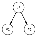
From our reasoning above, we know that $x_1 \perp\!\!\!\perp x_2 \mid \mu$, but that $x_1$ and $x_2$ are not unconditionally independent. This is true in general for any three variables in a graphical model in this configuration.

Exercise: mathematically prove the results stated above.

Solution: To show that $x_1$ and $x_2$ are not unconditionally independent, we must show that $p(x_1, x_2) \neq p(x_1)p(x_2)$. We can compute $p(x_1, x_2)$ by looking at the joint distribution over all three variables and then marginalizing over $\mu$:

Unfortunately, there is no way to factor the integral that separates terms with $x_1$ and terms with $x_2$, so this does not factor. In other words, in general, the integral above will not equal $p(x_1)p(x_2)$, so the variables are not unconditionally independent.

What about conditional independence given $\mu$? We need to show that $p(x_1, x_2\mid\mu) = p(x_1\mid\mu) p(x_2\mid\mu)$:

This mathematical result aligns with the intuition we built in the previous section.

Let’s look at another example:

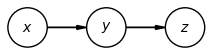
In this example, $x$ and $z$ are not unconditionally independent. Intuitively, we can see that $y$ depends on $x$, and $z$ depends on $y$, so that $x$ and $z$ are dependent.

But, $x$ and $z$ are conditionally independent given $y$: the lack of an arrow directly from $x$ to $z$ tells us that $z$ only depends on $x$ through $y$.

Exercise: mathematically prove the results stated above.

Let’s look at a third example:

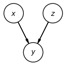
In this example, $x$ and $z$ are unconditionally independent, but given $y$, they are conditionally dependent. Why? Let’s look at an example that will help us build intuition for this result. Suppose that:

• $y$ is whether or not I have a stuffy nose.

• $x$ is whether or not I am sick (with a cold, flu, COVID, etc.)

• $z$ is whether or not I have seasonal allergies.

First, we can see that the description matches the graphical model: whether or not I have a stuffy nose depends on whether or not I’m sick, and whether or not I have allergies. But, sickness and allergies don’t affect each other. In other words, if I don’t know anything about whether I have a stuffy nose, then my sickness and allergies are independent of each other.

Now, suppose I wake up one morning with a stuffy nose (i.e., $y=1$), and I’m trying to determine whether I’m sick or have allergies. I look at the weather forecast, and see that the pollen counts are very high. As soon as I hear this information, I’m a lot more certain that $z=1$. But, even though the weather forecast didn’t directly tell me anything about whether or not I’m sick, my belief that I’m sick drops significantly: my symptoms have been explained away by the explanation that I probably have allergies.

In other words, conditioned on a value of $y$ (stuffy nose), knowing something about $z$ (allergies) gives me information about the distribution of $x$ (sickness). This is precisely the definition of conditional dependence.

Exercise: mathematically prove the results above.

These results can be formalized and generalized in the d-separation or Bayes’ ball algorithm. While this algorithm is beyond the scope of this textbook, we’ll look at a variant of it in a few chapters when we talk about causality.